6. Interaction
“A graphic is not ‘drawn’ once and for all; it is ‘constructed’ and reconstructed until it reveals all the relationships constituted by the interplay of the data. The best graphic operations are those carried out by the decision-maker themself.” — Jacques Bertin
Visualization provides a powerful means of making sense of data. A single image, however, typically provides answers to, at best, a handful of questions. Through interaction we can transform static images into tools for exploration: highlighting points of interest, zooming in to reveal finer-grained patterns, and linking across multiple views to reason about multi-dimensional relationships.
At the core of interaction is the notion of a selection: a means of indicating to the computer which elements or regions we are interested in. For example, we might hover the mouse over a point, click multiple marks, or draw a bounding box around a region to highlight subsets of the data for further scrutiny.
Alongside visual encodings and data transformations, Altair provides a selection abstraction for authoring interactions. These selections encompass three aspects:
Input event handling to select points or regions of interest, such as mouse hover, click, drag, scroll, and touch events.
Generalizing from the input to form a selection rule (or predicate) that determines whether or not a given data record lies within the selection.
Using the selection predicate to dynamically configure a visualization by driving conditional encodings, filter transforms, or scale domains.
This notebook introduces interactive selections and explores how to use them to author a variety of interaction techniques, such as dynamic queries, panning & zooming, details-on-demand, and brushing & linking.
This notebook is part of the data visualization curriculum.
import pandas as pd
import altair as alt
6.1. Datasets
We will visualize a variety of datasets from the vega-datasets collection:
A dataset of
carsfrom the 1970s and early 1980s,A dataset of
movies, previously used in the Data Transformation notebook,A dataset containing ten years of S&P 500 (
sp500) stock prices,A dataset of technology company
stocks, andA dataset of
flights, including departure time, distance, and arrival delay.
cars = 'https://cdn.jsdelivr.net/npm/vega-datasets@1/data/cars.json'
movies = 'https://cdn.jsdelivr.net/npm/vega-datasets@1/data/movies.json'
sp500 = 'https://cdn.jsdelivr.net/npm/vega-datasets@1/data/sp500.csv'
stocks = 'https://cdn.jsdelivr.net/npm/vega-datasets@1/data/stocks.csv'
flights = 'https://cdn.jsdelivr.net/npm/vega-datasets@1/data/flights-5k.json'
6.2. Introducing Selections
Let’s start with a basic selection: simply clicking a point to highlight it. Using the cars dataset, we’ll start with a scatter plot of horsepower versus miles per gallon, with a color encoding for the number cylinders in the car engine.
In addition, we’ll create a selection instance by calling alt.selection_single(), indicating we want a selection defined over a single value. By default, the selection uses a mouse click to determine the selected value. To register a selection with a chart, we must add it using the .add_selection() method.
Once our selection has been defined, we can use it as a parameter for conditional encodings, which apply a different encoding depending on whether a data record lies in or out of the selection. For example, consider the following code:
color=alt.condition(selection, 'Cylinders:O', alt.value('grey'))
This encoding definition states that data points contained within the selection should be colored according to the Cylinder field, while non-selected data points should use a default grey. An empty selection includes all data points, and so initially all points will be colored.
Try clicking different points in the chart below. What happens? (Click the background to clear the selection state and return to an “empty” selection.)
selection = alt.selection_single();

alt.Chart(cars).mark_circle().add_selection(
    selection
).encode(
    x='Horsepower:Q',
    y='Miles_per_Gallon:Q',
    color=alt.condition(selection, 'Cylinders:O', alt.value('grey')),
    opacity=alt.condition(selection, alt.value(0.8), alt.value(0.1))
)
Of course, highlighting individual data points one-at-a-time is not particularly exciting! As we’ll see, however, single value selections provide a useful building block for more powerful interactions. Moreover, single value selections are just one of the three selection types provided by Altair:
selection_single- select a single discrete value, by default on click events.selection_multi- select multiple discrete values. The first value is selected on mouse click and additional values toggled using shift-click.selection_interval- select a continuous range of values, initiated by mouse drag.
Let’s compare each of these selection types side-by-side. To keep our code tidy we’ll first define a function (plot) that generates a scatter plot specification just like the one above. We can pass a selection to the plot function to have it applied to the chart:
def plot(selection):
    return alt.Chart(cars).mark_circle().add_selection(
        selection
    ).encode(
        x='Horsepower:Q',
        y='Miles_per_Gallon:Q',
        color=alt.condition(selection, 'Cylinders:O', alt.value('grey')),
        opacity=alt.condition(selection, alt.value(0.8), alt.value(0.1))
    ).properties(
        width=240,
        height=180
    )
Let’s use our plot function to create three chart variants, one per selection type.
The first (single) chart replicates our earlier example. The second (multi) chart supports shift-click interactions to toggle inclusion of multiple points within the selection. The third (interval) chart generates a selection region (or brush) upon mouse drag. Once created, you can drag the brush around to select different points, or scroll when the cursor is inside the brush to scale (zoom) the brush size.
Try interacting with each of the charts below!
alt.hconcat(
  plot(alt.selection_single()).properties(title='Single (Click)'),
  plot(alt.selection_multi()).properties(title='Multi (Shift-Click)'),
  plot(alt.selection_interval()).properties(title='Interval (Drag)')
)
The examples above use default interactions (click, shift-click, drag) for each selection type. We can further customize the interactions by providing input event specifications using Vega event selector syntax. For example, we can modify our single and multi charts to trigger upon mouseover events instead of click events.
Hold down the shift key in the second chart to “paint” with data!
alt.hconcat(
  plot(alt.selection_single(on='mouseover')).properties(title='Single (Mouseover)'),
  plot(alt.selection_multi(on='mouseover')).properties(title='Multi (Shift-Mouseover)')
)
Now that we’ve covered the basics of Altair selections, let’s take a tour through the various interaction techniques they enable!
6.3. Dynamic Queries
Dynamic queries enables rapid, reversible exploration of data to isolate patterns of interest. As defined by Ahlberg, Williamson, & Shneiderman, a dynamic query:
represents a query graphically,
provides visible limits on the query range,
provides a graphical representation of the data and query result,
gives immediate feedback of the result after every query adjustment,
and allows novice users to begin working with little training.
A common approach is to manipulate query parameters using standard user interface widgets such as sliders, radio buttons, and drop-down menus. To generate dynamic query widgets, we can apply a selection’s bind operation to one or more data fields we wish to query.
Let’s build an interactive scatter plot that uses a dynamic query to filter the display. Given a scatter plot of movie ratings (from Rotten Tomates and IMDB), we can add a selection over the Major_Genre field to enable interactive filtering by film genre.
To start, let’s extract the unique (non-null) genres from the movies data:
df = pd.read_json(movies) # load movies data
genres = df['Major_Genre'].unique() # get unique field values
genres = list(filter(lambda d: d is not None, genres)) # filter out None values
genres.sort() # sort alphabetically
For later use, let’s also define a list of unique MPAA_Rating values:
mpaa = ['G', 'PG', 'PG-13', 'R', 'NC-17', 'Not Rated']
Now let’s create a single selection bound to a drop-down menu.
Use the dynamic query menu below to explore the data. How do ratings vary by genre? How would you revise the code to filter MPAA_Rating (G, PG, PG-13, etc.) instead of Major_Genre?
selectGenre = alt.selection_single(
    name='Select', # name the selection 'Select'
    fields=['Major_Genre'], # limit selection to the Major_Genre field
    init={'Major_Genre': genres[0]}, # use first genre entry as initial value
    bind=alt.binding_select(options=genres) # bind to a menu of unique genre values
)

alt.Chart(movies).mark_circle().add_selection(
    selectGenre
).encode(
    x='Rotten_Tomatoes_Rating:Q',
    y='IMDB_Rating:Q',
    tooltip='Title:N',
    opacity=alt.condition(selectGenre, alt.value(0.75), alt.value(0.05))
)
Our construction above leverages multiple aspects of selections:
We give the selection a name (
'Select'). This name is not required, but allows us to influence the label text of the generated dynamic query menu. (What happens if you remove the name? Try it!)We constrain the selection to a specific data field (
Major_Genre). Earlier when we used asingleselection, the selection mapped to individual data points. By limiting the selection to a specific field, we can select all data points whoseMajor_Genrefield value matches the single selected value.We initialize
init=...the selection to a starting value.We
bindthe selection to an interface widget, in this case a drop-down menu viabinding_select.As before, we then use a conditional encoding to control the opacity channel.
6.3.1. Binding Selections to Multiple Inputs
One selection instance can be bound to multiple dynamic query widgets. Let’s modify the example above to provide filters for both Major_Genre and MPAA_Rating, using radio buttons instead of a menu. Our single selection is now defined over a single pair of genre and MPAA rating values
Look for surprising conjunctions of genre and rating. Are there any G or PG-rated horror films?
# single-value selection over [Major_Genre, MPAA_Rating] pairs
# use specific hard-wired values as the initial selected values
selection = alt.selection_single(
    name='Select',
    fields=['Major_Genre', 'MPAA_Rating'],
    init={'Major_Genre': 'Drama', 'MPAA_Rating': 'R'},
    bind={'Major_Genre': alt.binding_select(options=genres), 'MPAA_Rating': alt.binding_radio(options=mpaa)}
)

# scatter plot, modify opacity based on selection
alt.Chart(movies).mark_circle().add_selection(
    selection
).encode(
    x='Rotten_Tomatoes_Rating:Q',
    y='IMDB_Rating:Q',
    tooltip='Title:N',
    opacity=alt.condition(selection, alt.value(0.75), alt.value(0.05))
)
Fun facts: The PG-13 rating didn’t exist when the movies Jaws and Jaws 2 were released. The first film to receive a PG-13 rating was 1984’s Red Dawn.
6.3.2. Using Visualizations as Dynamic Queries
Though standard interface widgets show the possible query parameter values, they do not visualize the distribution of those values. We might also wish to use richer interactions, such as multi-value or interval selections, rather than input widgets that select only a single value at a time.
To address these issues, we can author additional charts to both visualize data and support dynamic queries. Let’s add a histogram of the count of films per year and use an interval selection to dynamically highlight films over selected time periods.
Interact with the year histogram to explore films from different time periods. Do you seen any evidence of sampling bias across the years? (How do year and critics’ ratings relate?)
The years range from 1930 to 2040! Are future films in pre-production, or are there “off-by-one century” errors? Also, depending on which time zone you’re in, you may see a small bump in either 1969 or 1970. Why might that be? (See the end of the notebook for an explanation!)
brush = alt.selection_interval(
    encodings=['x'] # limit selection to x-axis (year) values
)

# dynamic query histogram
years = alt.Chart(movies).mark_bar().add_selection(
    brush
).encode(
    alt.X('year(Release_Date):T', title='Films by Release Year'),
    alt.Y('count():Q', title=None)
).properties(
    width=650,
    height=50
)

# scatter plot, modify opacity based on selection
ratings = alt.Chart(movies).mark_circle().encode(
    x='Rotten_Tomatoes_Rating:Q',
    y='IMDB_Rating:Q',
    tooltip='Title:N',
    opacity=alt.condition(brush, alt.value(0.75), alt.value(0.05))
).properties(
    width=650,
    height=400
)

alt.vconcat(years, ratings).properties(spacing=5)
The example above provides dynamic queries using a linked selection between charts:
We create an
intervalselection (brush), and setencodings=['x']to limit the selection to the x-axis only, resulting in a one-dimensional selection interval.We register
brushwith our histogram of films per year via.add_selection(brush).We use
brushin a conditional encoding to adjust the scatter plotopacity.
This interaction technique of selecting elements in one chart and seeing linked highlights in one or more other charts is known as brushing & linking.
6.4. Panning & Zooming
The movie rating scatter plot is a bit cluttered in places, making it hard to examine points in denser regions. Using the interaction techniques of panning and zooming, we can inspect dense regions more closely.
Let’s start by thinking about how we might express panning and zooming using Altair selections. What defines the “viewport” of a chart? Axis scale domains!
We can change the scale domains to modify the visualized range of data values. To do so interactively, we can bind an interval selection to scale domains with the code bind='scales'. The result is that instead of an interval brush that we can drag and zoom, we instead can drag and zoom the entire plotting area!
In the chart below, click and drag to pan (translate) the view, or scroll to zoom (scale) the view. What can you discover about the precision of the provided rating values?
alt.Chart(movies).mark_circle().add_selection(
    alt.selection_interval(bind='scales')
).encode(
    x='Rotten_Tomatoes_Rating:Q',
    y=alt.Y('IMDB_Rating:Q', axis=alt.Axis(minExtent=30)), # use min extent to stabilize axis title placement
    tooltip=['Title:N', 'Release_Date:N', 'IMDB_Rating:Q', 'Rotten_Tomatoes_Rating:Q']
).properties(
    width=600,
    height=400
)
Zooming in, we can see that the rating values have limited precision! The Rotten Tomatoes ratings are integers, while the IMDB ratings are truncated to tenths. As a result, there is overplotting even when we zoom, with multiple movies sharing the same rating values.
Reading the code above, you may notice the code alt.Axis(minExtent=30) in the y encoding channel. The minExtent parameter ensures a minimum amount of space is reserved for axis ticks and labels. Why do this? When we pan and zoom, the axis labels may change and cause the axis title position to shift. By setting a minimum extent we can reduce distracting movements in the plot. Try changing the minExtent value, for example setting it to zero, and then zoom out to see what happens when longer axis labels enter the view.
Altair also includes a shorthand for adding panning and zooming to a plot. Instead of directly creating a selection, you can call .interactive() to have Altair automatically generate an interval selection bound to the chart’s scales:
alt.Chart(movies).mark_circle().encode(
    x='Rotten_Tomatoes_Rating:Q',
    y=alt.Y('IMDB_Rating:Q', axis=alt.Axis(minExtent=30)), # use min extent to stabilize axis title placement
    tooltip=['Title:N', 'Release_Date:N', 'IMDB_Rating:Q', 'Rotten_Tomatoes_Rating:Q']
).properties(
    width=600,
    height=400
).interactive()
By default, scale bindings for selections include both the x and y encoding channels. What if we want to limit panning and zooming along a single dimension? We can invoke encodings=['x'] to constrain the selection to the x channel only:
alt.Chart(movies).mark_circle().add_selection(
    alt.selection_interval(bind='scales', encodings=['x'])
).encode(
    x='Rotten_Tomatoes_Rating:Q',
    y=alt.Y('IMDB_Rating:Q', axis=alt.Axis(minExtent=30)), # use min extent to stabilize axis title placement
    tooltip=['Title:N', 'Release_Date:N', 'IMDB_Rating:Q', 'Rotten_Tomatoes_Rating:Q']
).properties(
    width=600,
    height=400
)
When zooming along a single axis only, the shape of the visualized data can change, potentially affecting our perception of relationships in the data. Choosing an appropriate aspect ratio is an important visualization design concern!
6.6. Details on Demand
Once we spot points of interest within a visualization, we often want to know more about them. Details-on-demand refers to interactively querying for more information about selected values. Tooltips are one useful means of providing details on demand. However, tooltips typically only show information for one data point at a time. How might we show more?
The movie ratings scatterplot includes a number of potentially interesting outliers where the Rotten Tomatoes and IMDB ratings disagree. Let’s create a plot that allows us to interactively select points and show their labels. To trigger the filter query on either the hover or click interaction, we will use the Altair composition operator | (“or”).
Mouse over points in the scatter plot below to see a highlight and title label. Shift-click points to make annotations persistent and view multiple labels at once. Which movies are loved by Rotten Tomatoes critics, but not the general audience on IMDB (or vice versa)? See if you can find possible errors, where two different movies with the same name were accidentally combined!
hover = alt.selection_single(
    on='mouseover',  # select on mouseover
    nearest=True,    # select nearest point to mouse cursor
    empty='none'     # empty selection should match nothing
)

click = alt.selection_multi(
    empty='none' # empty selection matches no points
)

# scatter plot encodings shared by all marks
plot = alt.Chart().mark_circle().encode(
    x='Rotten_Tomatoes_Rating:Q',
    y='IMDB_Rating:Q'
)

# shared base for new layers
base = plot.transform_filter(
    hover | click # filter to points in either selection
)

# layer scatter plot points, halo annotations, and title labels
alt.layer(
    plot.add_selection(hover).add_selection(click),
    base.mark_point(size=100, stroke='firebrick', strokeWidth=1),
    base.mark_text(dx=4, dy=-8, align='right', stroke='white', strokeWidth=2).encode(text='Title:N'),
    base.mark_text(dx=4, dy=-8, align='right').encode(text='Title:N'),
    data=movies
).properties(
    width=600,
    height=450
)
The example above adds three new layers to the scatter plot: a circular annotation, white text to provide a legible background, and black text showing a film title. In addition, this example uses two selections in tandem:
A single selection (
hover) that includesnearest=Trueto automatically select the nearest data point as the mouse moves.A multi selection (
click) to create persistent selections via shift-click.
Both selections include the set empty='none' to indicate that no points should be included if a selection is empty. These selections are then combined into a single filter predicate — the logical or of hover and click — to include points that reside in either selection. We use this predicate to filter the new layers to show annotations and labels for selected points only.
Using selections and layers, we can realize a number of different designs for details on demand! For example, here is a log-scaled time series of technology stock prices, annotated with a guideline and labels for the date nearest the mouse cursor:
# select a point for which to provide details-on-demand
label = alt.selection_single(
    encodings=['x'], # limit selection to x-axis value
    on='mouseover',  # select on mouseover events
    nearest=True,    # select data point nearest the cursor
    empty='none'     # empty selection includes no data points
)

# define our base line chart of stock prices
base = alt.Chart().mark_line().encode(
    alt.X('date:T'),
    alt.Y('price:Q', scale=alt.Scale(type='log')),
    alt.Color('symbol:N')
)

alt.layer(
    base, # base line chart

    # add a rule mark to serve as a guide line
    alt.Chart().mark_rule(color='#aaa').encode(
        x='date:T'
    ).transform_filter(label),

    # add circle marks for selected time points, hide unselected points
    base.mark_circle().encode(
        opacity=alt.condition(label, alt.value(1), alt.value(0))
    ).add_selection(label),

    # add white stroked text to provide a legible background for labels
    base.mark_text(align='left', dx=5, dy=-5, stroke='white', strokeWidth=2).encode(
        text='price:Q'
    ).transform_filter(label),

    # add text labels for stock prices
    base.mark_text(align='left', dx=5, dy=-5).encode(
        text='price:Q'
    ).transform_filter(label),

    data=stocks
).properties(
    width=700,
    height=400
)
Putting into action what we’ve learned so far: can you modify the movie scatter plot above (the one with the dynamic query over years) to include a rule mark that shows the average IMDB (or Rotten Tomatoes) rating for the data contained within the year interval selection?
6.7. Brushing & Linking, Revisited
Earlier in this notebook we saw an example of brushing & linking: using a dynamic query histogram to highlight points in a movie rating scatter plot. Here, we’ll visit some additional examples involving linked selections.
Returning to the cars dataset, we can use the repeat operator to build a scatter plot matrix (SPLOM) that shows associations between mileage, acceleration, and horsepower. We can define an interval selection and include it within our repeated scatter plot specification to enable linked selections among all the plots.
Click and drag in any of the plots below to perform brushing & linking!
brush = alt.selection_interval(
    resolve='global' # resolve all selections to a single global instance
)

alt.Chart(cars).mark_circle().add_selection(
    brush
).encode(
    alt.X(alt.repeat('column'), type='quantitative'),
    alt.Y(alt.repeat('row'), type='quantitative'),
    color=alt.condition(brush, 'Cylinders:O', alt.value('grey')),
    opacity=alt.condition(brush, alt.value(0.8), alt.value(0.1))
).properties(
    width=140,
    height=140
).repeat(
    column=['Acceleration', 'Horsepower', 'Miles_per_Gallon'],
    row=['Miles_per_Gallon', 'Horsepower', 'Acceleration']
)
Note above the use of resolve='global' on the interval selection. The default setting of 'global' indicates that across all plots only one brush can be active at a time. However, in some cases we might want to define brushes in multiple plots and combine the results. If we use resolve='union', the selection will be the union of all brushes: if a point resides within any brush it will be selected. Alternatively, if we use resolve='intersect', the selection will consist of the intersection of all brushes: only points that reside within all brushes will be selected.
Try setting the resolve parameter to 'union' and 'intersect' and see how it changes the resulting selection logic.
6.7.1. Cross-Filtering
The brushing & linking examples we’ve looked at all use conditional encodings, for example to change opacity values in response to a selection. Another option is to use a selection defined in one view to filter the content of another view.
Let’s build a collection of histograms for the flights dataset: arrival delay (how early or late a flight arrives, in minutes), distance flown (in miles), and time of departure (hour of the day). We’ll use the repeat operator to create the histograms, and add an interval selection for the x axis with brushes resolved via intersection.
In particular, each histogram will consist of two layers: a gray background layer and a blue foreground layer, with the foreground layer filtered by our intersection of brush selections. The result is a cross-filtering interaction across the three charts!
Drag out brush intervals in the charts below. As you select flights with longer or shorter arrival delays, how do the distance and time distributions respond?
brush = alt.selection_interval(
    encodings=['x'],
    resolve='intersect'
);

hist = alt.Chart().mark_bar().encode(
    alt.X(alt.repeat('row'), type='quantitative',
        bin=alt.Bin(maxbins=100, minstep=1), # up to 100 bins
        axis=alt.Axis(format='d', titleAnchor='start') # integer format, left-aligned title
    ),
    alt.Y('count():Q', title=None) # no y-axis title
)

alt.layer(
    hist.add_selection(brush).encode(color=alt.value('lightgrey')),
    hist.transform_filter(brush)
).properties(
    width=900,
    height=100
).repeat(
    row=['delay', 'distance', 'time'],
    data=flights
).transform_calculate(
    delay='datum.delay < 180 ? datum.delay : 180', # clamp delays > 3 hours
    time='hours(datum.date) + minutes(datum.date) / 60' # fractional hours
).configure_view(
    stroke='transparent' # no outline
)
By cross-filtering you can observe that delayed flights are more likely to depart at later hours. This phenomenon is familiar to frequent fliers: a delay can propagate through the day, affecting subsequent travel by that plane. For the best odds of an on-time arrival, book an early flight!
The combination of multiple views and interactive selections can enable valuable forms of multi-dimensional reasoning, turning even basic histograms into powerful input devices for asking questions of a dataset!
6.8. Summary
For more information about the supported interaction options in Altair, please consult the Altair interactive selection documentation. For details about customizing event handlers, for example to compose multiple interaction techniques or support touch-based input on mobile devices, see the Vega-Lite selection documentation.
Interested in learning more?
The selection abstraction was introduced in the paper Vega-Lite: A Grammar of Interactive Graphics, by Satyanarayan, Moritz, Wongsuphasawat, & Heer.
The PRIM-9 system (for projection, rotation, isolation, and masking in up to 9 dimensions) is one of the earliest interactive visualization tools, built in the early 1970s by Fisherkeller, Tukey, & Friedman. A retro demo video survives!
The concept of brushing & linking was crystallized by Becker, Cleveland, & Wilks in their 1987 article Dynamic Graphics for Data Analysis.
For a comprehensive summary of interaction techniques for visualization, see Interactive Dynamics for Visual Analysis by Heer & Shneiderman.
Finally, for a treatise on what makes interaction effective, read the classic Direct Manipulation Interfaces paper by Hutchins, Hollan, & Norman.
6.8.1. Appendix: On The Representation of Time
Earlier we observed a small bump in the number of movies in either 1969 and 1970. Where does that bump come from? And why 1969 or 1970? The answer stems from a combination of missing data and how your computer represents time.
Internally, dates and times are represented relative to the UNIX epoch, in which time “zero” corresponds to the stroke of midnight on January 1, 1970 in UTC time, which runs along the prime meridian. It turns out there are a few movies with missing (null) release dates. Those null values get interpreted as time 0, and thus map to January 1, 1970 in UTC time. If you live in the Americas – and thus in “earlier” time zones – this precise point in time corresponds to an earlier hour on December 31, 1969 in your local time zone. On the other hand, if you live near or east of the prime meridian, the date in your local time zone will be January 1, 1970.
The takeaway? Always be skeptical of your data, and be mindful that how data is represented (whether as date times, or floating point numbers, or latitudes and longitudes, etc.) can sometimes lead to artifacts that impact analysis!